THE SOLENOID
`color{blue} ✍️` The solenoid and the toroid are two pieces of equipment which generate magnetic fields. The television uses the solenoid to generate magnetic fields needed.
`color{blue} ✍️` The synchrotron uses a combination of both to generate the high magnetic fields required. In both, solenoid and toroid, we come across a situation of high symmetry where Ampere’s law can be conveniently applied.
`color{brown}bb ul("The solenoid")`
`color{blue} ✍️` We shall discuss a long solenoid. By long solenoid we mean that the solenoid’s length is large compared to its radius. It consists of a long wire wound in the form of a helix where the neighbouring turns are closely spaced.
`color {blue}{➢➢}` So each turn can be regarded as a circular loop. The net magnetic field is the vector sum of the fields due to all the turns. Enamelled wires are used for winding so that turns are insulated from each other.
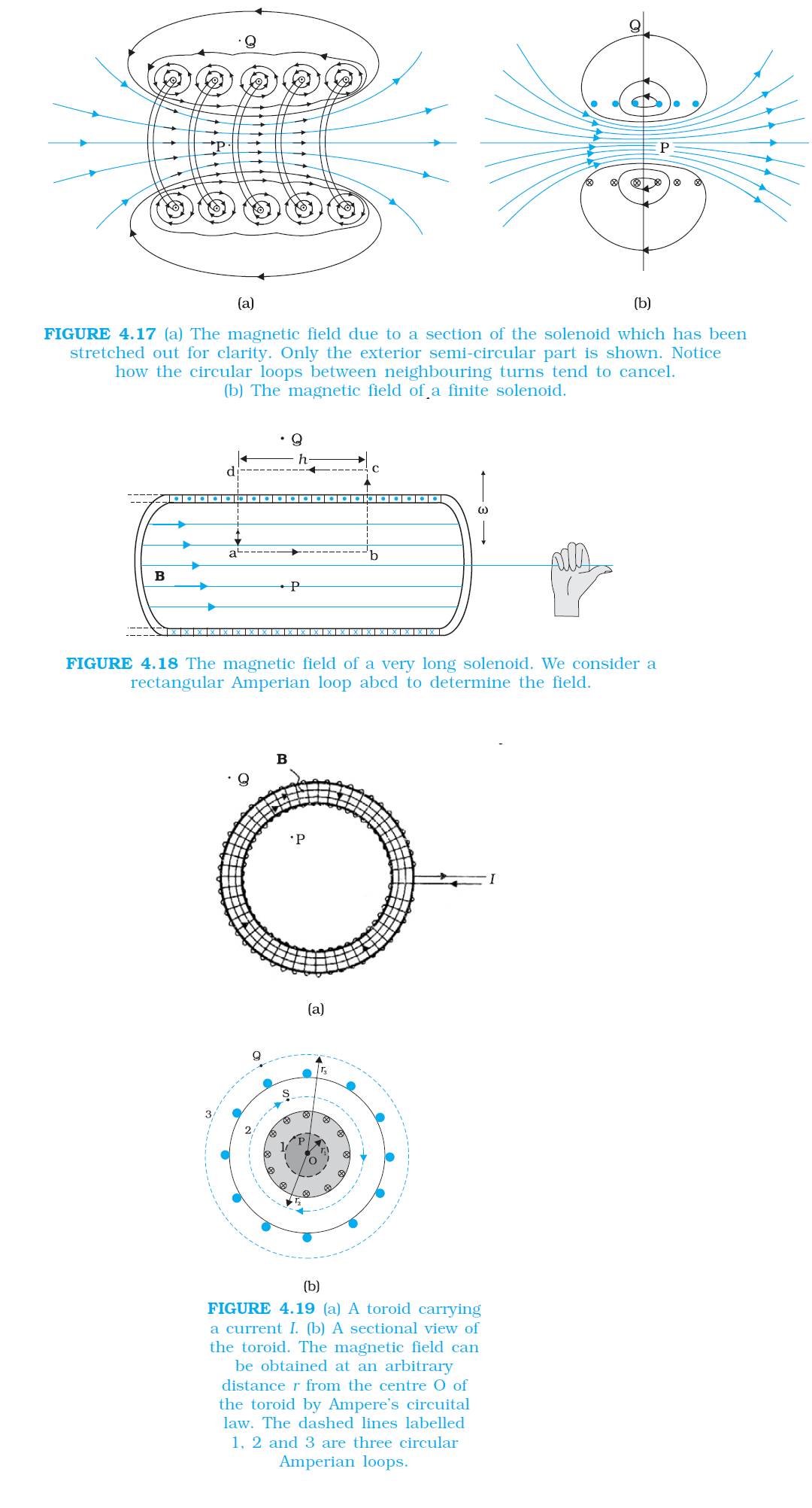
`color {blue}{➢➢}`Figure 4.17 displays the magnetic field lines for a finite solenoid. We show a section of this solenoid in an enlarged manner in Fig. 4.17(a). Figure 4.17(b) shows the entire finite solenoid with its magnetic field. In Fig. 4.17(a), it is clear from the circular loops that the field between two neighbouring turns vanishes. In Fig. 4.17(b),
`color{blue} ✍️` we see that the field at the interior mid-point `P` is uniform, strong and along the axis of the solenoid.
`color {blue}{➢➢}` The field at the exterior mid-point `Q` is weak and moreover is along the axis of the solenoid with no perpendicular or normal component. As the solenoid is made longer it appears like a long cylindrical metal sheet.
`color{blue} ✍️` Figure 4.18 represents this idealised picture. The field outside the solenoid approaches zero. We shall assume that the field outside is zero. The field inside becomes everywhere parallel to the axis.

`color{blue} ✍️` Consider a rectangular Amperian loop abcd. Along `cd` the field is zero as argued above. Along transverse sections `bc` and `ad`, the field component is zero. Thus, these two sections make no contribution. Let the field along ab be `B`.
`color {blue}{➢➢}` Thus, the relevant length of the Amperian loop is, `L = h`. Let `n` be the number of turns per unit length, then the total number of turns is `nh`. The enclosed current is, `I_e = I (n h),` where` I` is the current in the solenoid. From Ampere’s circuital law [Eq. 4.17 (b)]
`color{blue}(BL = mu_0I_e " ", Bh = mu_0 I(n h))`
`color{blue} ✍️` The direction of the field is given by the right-hand rule. The solenoid is commonly used to obtain a uniform magnetic field. We shall see in the next chapter that a large field is possible by inserting a soft iron core inside the solenoid.
`color{blue} ✍️` The synchrotron uses a combination of both to generate the high magnetic fields required. In both, solenoid and toroid, we come across a situation of high symmetry where Ampere’s law can be conveniently applied.
`color{brown}bb ul("The solenoid")`
`color{blue} ✍️` We shall discuss a long solenoid. By long solenoid we mean that the solenoid’s length is large compared to its radius. It consists of a long wire wound in the form of a helix where the neighbouring turns are closely spaced.
`color {blue}{➢➢}` So each turn can be regarded as a circular loop. The net magnetic field is the vector sum of the fields due to all the turns. Enamelled wires are used for winding so that turns are insulated from each other.
`color {blue}{➢➢}`Figure 4.17 displays the magnetic field lines for a finite solenoid. We show a section of this solenoid in an enlarged manner in Fig. 4.17(a). Figure 4.17(b) shows the entire finite solenoid with its magnetic field. In Fig. 4.17(a), it is clear from the circular loops that the field between two neighbouring turns vanishes. In Fig. 4.17(b),
`color{blue} ✍️` we see that the field at the interior mid-point `P` is uniform, strong and along the axis of the solenoid.
`color {blue}{➢➢}` The field at the exterior mid-point `Q` is weak and moreover is along the axis of the solenoid with no perpendicular or normal component. As the solenoid is made longer it appears like a long cylindrical metal sheet.
`color{blue} ✍️` Figure 4.18 represents this idealised picture. The field outside the solenoid approaches zero. We shall assume that the field outside is zero. The field inside becomes everywhere parallel to the axis.
`color{blue} ✍️` Consider a rectangular Amperian loop abcd. Along `cd` the field is zero as argued above. Along transverse sections `bc` and `ad`, the field component is zero. Thus, these two sections make no contribution. Let the field along ab be `B`.
`color {blue}{➢➢}` Thus, the relevant length of the Amperian loop is, `L = h`. Let `n` be the number of turns per unit length, then the total number of turns is `nh`. The enclosed current is, `I_e = I (n h),` where` I` is the current in the solenoid. From Ampere’s circuital law [Eq. 4.17 (b)]
`color{blue}(BL = mu_0I_e " ", Bh = mu_0 I(n h))`
`color{blue}(B = μ_0 n I)`
...........(4.20)`color{blue} ✍️` The direction of the field is given by the right-hand rule. The solenoid is commonly used to obtain a uniform magnetic field. We shall see in the next chapter that a large field is possible by inserting a soft iron core inside the solenoid.